


자동제어 | 근궤적선도 |
페이지 정보
작성자 cemtool 작성일14-04-22 13:24 조회18,258회 댓글0건본문
다음의 전달함수를 가진 시스템을 생각해보자.
«풀이»
- ex6_15.cem
/* Root-locus plot */
num = [1 1];
K = 0:100:0.5;
// a = 10den1 = [1 10 0 0];
rlocus(num, den1, K);
title("Root-Locus Plot of G(s) = K(s + 1)/[s^2 (s + 10)]")// a = 9figureden2 = [1 9 0 0];
rlocus(num, den2, K);
title("Root-Locus Plot of G(s) = K(s + 1)/[s^2 (s + 9)]")// a = 8figureden3 = [1 8 0 0];
rlocus(num, den3, K);
title("Root-Locus Plot of G(s) = K(s + 1)/[s^2 (s + 8)]")// a = 3figureden4 = [1 3 0 0];
rlocus(num, den4, K);
title("Root-Locus Plot of G(s) = K(s + 1)/[s^2 (s + 3)]")// a = 1figureden5 = [1 1 0 0];
rlocus(num, den5, K);
title("Root-Locus Plot of G(s) = K(s + 1)/[s^2 (s + 1)]")
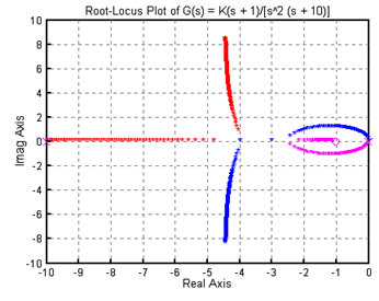
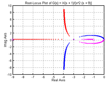
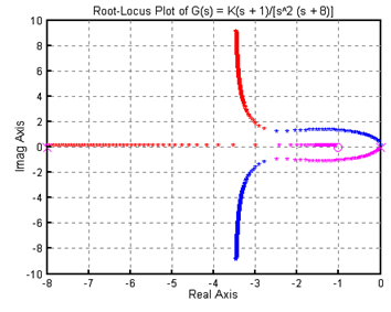
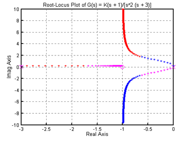
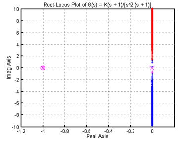
결과를 다음과 같이 요약할 수 있다.
(a) a=10일 때 :  이탈점 s=-2.5와 s=-4.0
(b) a=9일 때  :  두 개의 이탈점이 s=-3 의 한 점으로 수렴한다.
(c) a=8일 때  :  s=0 을 제외하고 이탈점이 없다.
(d) a=3일 때  :  근궤적선도가 상당히 오른쪽으로 밀려난다.
(e) a=1일 때  :  영점과 극점이 상쇄되고, 근궤적선도는 허수축에 그려진다.
댓글목록
등록된 댓글이 없습니다.